Learning about Rust Benchmarking with Sudoku from 5 minutes to 17 seconds
I’ll take you through the process of optimizing a Sudoku solver written in Rust. We’ll start with a simple, unoptimized version and apply a series of optimizations that will take the time to solve 100,000 puzzles from over 5 minutes down to just 33 seconds, and 20,000 of the hardest puzzles from over 2 minutes down to just 17 seconds.
The Setup
The project is a command-line Sudoku solver written in Rust. The puzzles are read from text files in the src/puzzle_banks directory, thanks to the github project Sudoku Exchange Puzzle Bank. Each line in these files represents a single puzzle in the following format:
0000847b216e 020900000048000031000063020009407003003080200400105600030570000250000180000006050 2.3The second part of the line is the puzzle itself, where 0 represents an empty cell.
The basic flow of the program is:
- Read the puzzle file.
- For each line, parse the puzzle string into a
Boardstruct. - Call the
solvefunction on the board. - Print the statistics.
The Benchmarks
Here is a summary of the benchmarks for both the “Easy” and “Diabolical” puzzle sets:
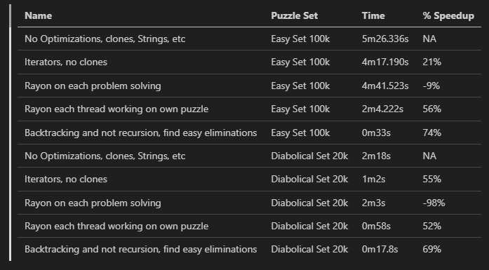
The Initial State: A Simple Backtracking Solver
Our starting point was a straightforward backtracking solver. The solver would recursively try to place valid numbers in empty cells. If a path led to a dead end, it would backtrack and try a different number.
While this approach worked, it was slow. The initial benchmark for solving 100,000 easy puzzles was 5 minutes and 26 seconds, and 20,000 of the hardest puzzles took 2 minutes and 18 seconds. The main culprits for this slow performance were:
- Excessive Cloning: The board state was cloned for every single step of the recursion.
- Frequent Allocations: Functions that fetched rows, columns, and sections of the board were returning new vectors (
Vecs), leading to frequent memory allocations.
Here is what the initial solve function looked like:
pub fn solve(mut board: Board) -> Result<Board, String> {
    // Find the first empty cell
    for row in 0..board.height() {
        for col in 0..board.width() {
            if board.get_cell(row, col).is_some() {
                continue;
            }
            // Get valid options for this cell
            let options = board.get_options(row, col);
if let Some(option_values) = options {
                // Try each valid option
                for val in option_values {
                    // Place the value
                    board.set_cell(row, col, Some(val));
                    // Recursively try to solve the rest
                    match solve(board.clone()) { // The expensive clone!
                        Ok(solved) => return Ok(solved), // Found solution!
                        Err(_) => {
                            // This path didn't work, backtrack
                            board.set_cell(row, col, None);
                            // Continue to next option
                        }
                    }
                }
                // No valid options worked, backtrack
                return Err("No valid solution from this state".to_string());
            } else {
                // No options available for this empty cell - dead end
                return Err("No options available".to_string());
            }
        }
    }
    // If we get here, all cells are filled - puzzle is solved!
    Ok(board)
}
First Optimization: Reducing Allocations and Clones
The first step was to reduce the memory overhead. We did this by:
- Removing
board.clone(): Instead of cloning the board for each recursive call, we modified thesolvefunction to use a mutable reference (&mut Board). This single change had a huge impact on performance.
Before:
match solve(board.clone()) { ... }After:
if solve(board).is_ok() { ... }- Using Iterators: The
get_row,get_col, andget_sectionfunctions were refactored to return iterators instead of new vectors. This avoided unnecessary memory allocations. - Before:
pub fn get_row(&self, row: usize) -> Vec<Option<NonZeroU8>> {
        ...
        self.cells[start..end].to_vec()
}- After:
pub fn get_row(&self, row: usize) -> &[Option<NonZeroU8>] {
        ...
        &self.cells[start..end]
}- Optimizing Option Lookups: The
get_optionsfunction, which finds valid numbers for a cell, was optimized to use a boolean array for faster lookups, instead of searching through vectors. - Before:
let options: Vec<NonZeroU8> = (1..=self.max_value.get())
        .filter_map(|u| NonZeroU8::new(u))
        .filter(|x| {
            !row_values.contains(x) && !col_values.contains(x) && !section_values.contains(x)
        })
.collect();- After:
let mut used = vec![false; self.max_value.get() as usize + 1];
    // ... populate used array ...
    let options: Vec<NonZeroU8> = (1..=self.max_value.get())
        .filter_map(|u| {
            if used[u as usize] {
                None
            } else {
                NonZeroU8::new(u)
            }
        })
        .collect();
These changes resulted in a 21% speedup on the easy puzzles and a 55% speedup on the diabolical puzzles. This shows that reducing memory allocations is even more important for harder problems, likely because the recursion depth is much greater, and the overhead of cloning larger and more complex board states adds up.
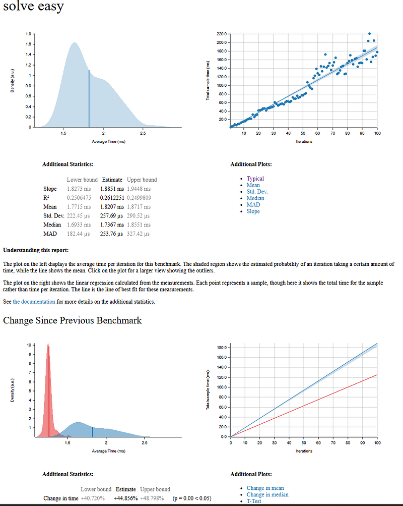
Criterion
I really wanted to use Criterion for my first time to better get a view into how each puzzle is being solved. Here is a set up of criterion running a single puzzle 5000 times with its code. Notice that each cycle is around 1.25 ms.
use criterion::{black_box, criterion_group, criterion_main, Criterion};
use sudoku_solver::{Board, solve};
fn criterion_benchmark(c: &mut Criterion) {
let puzzle = "050703060007000800000816000000030000005000100730040086906000204840572093000409000";
c.bench_function("solve easy", |b| {
b.iter(|| {
let mut board = Board::from_puzzle_bank_line(&format!("id {} 1.2", puzzle)).unwrap();
solve(black_box(&mut board))
})
});
}criterion_group!(benches, criterion_benchmark);
criterion_main!(benches);
Criterion Benchmarks for the first
Parallelism with Rayon
The next step was to introduce parallelism using the rayon crate.
Attempt 1: Parallelizing the Solver
Our first attempt was to parallelize the solver itself. The idea was to explore different solution paths in parallel. However, this resulted in a 9% slowdown on the easy puzzles and a staggering 98% slowdown on the diabolical puzzles. The overhead of managing parallel tasks and the re-introduction of some cloning outweighed the benefits, especially for the harder puzzles which have a deeper recursion space and require more coordination between threads.
pub fn solve(board: &mut Board) -> Result<(), String> {
    // ...
    let solution = options
        .into_par_iter() // Parallel iteration
        .find_map_any(|val| {
            let mut new_board = board.clone(); // Cloning is back!
            new_board.set_cell(row, col, Some(val));
            if solve_sequential(&mut new_board).is_ok() {
                Some(new_board)
            } else {
                None
            }
        });
    // ...
}
And criterion shows the same regression. I think the skew and larger variance in the benchmark is the most noticable that we are hitting non-deterministic data sharing between the threads. Turns out that parallel code can easily make your code slower if you’re not thinking.
Attempt 2: Parallelizing the Puzzle Set
The second, more successful approach was to solve multiple puzzles in parallel. We used rayon to distribute the puzzles from the input file across multiple threads. Each thread would then solve one puzzle sequentially.
use rayon::prelude::*;
fn main() {
    // ...
    let results: Vec<Result<(), String>> = contents
        .par_lines() // Parallel iteration over lines
        .filter(|line| !line.trim().is_empty())
        .map(|line| {
            let mut board = Board::from_puzzle_bank_line(line)?;
            solve(&mut board)
        })
        .collect();
    // ...
}
This “embarrassingly parallel” approach was very effective, resulting in a 56% speedup on the easy puzzles and a 52% speedup on the diabolical puzzles. The benchmark iteration is looking much better. Something to note is that the time to solve the puzzle has not changed much since the first solution, but we are using parallelism of the cpu cores better.

The Big Breakthrough: Constraint Propagation
The most significant performance gain came from improving the solver’s logic. Instead of immediately resorting to backtracking, we first added a logical deduction step.
We implemented an eliminate function that repeatedly scans the board for “naked singles” – empty cells that have only one possible valid number. When it finds one, it fills it in. It keeps scanning and filling until it can’t find any more naked singles.
fn eliminate(board: &mut Board) -> bool {
    let mut made_change = true;
    while made_change {
        made_change = false;
        for row in 0..board.height() {
            for col in 0..board.width() {
                if board.get_cell(row, col).is_some() {
                    continue;
                }
                if let Some(options) = board.get_options(row, col) {
                    if options.len() == 1 {
                        board.set_cell(row, col, Some(options[0]));
                        made_change = true;
                    }
                }
            }
        }
    }
    // ... check if solved ...
}
The main solve function now first calls eliminate. Only if the puzzle is not solved by logic alone does it proceed to the backtracking algorithm.
pub fn solve(board: &mut Board) -> Result<(), String> {
    if eliminate(board) {
        return Ok(());
    }
    solve_backtracking(board)
}
This is a form of constraint propagation, and it dramatically prunes the search space for the backtracking solver. This change brought the time down to an incredible 33 seconds for the easy puzzles (a 74% improvement) and 17.8 seconds for the diabolical puzzles (a 69% improvement). The benchmark now shows that the new improvements to the algorithm is significantly improving the time to solve a single puzzle, changing from 1.2 ms to 46 µs.
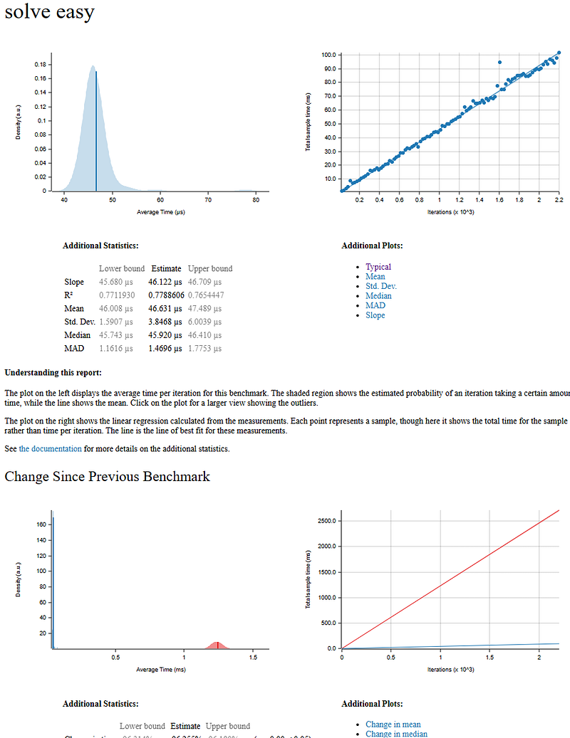
It’s important to clarify a common point of confusion: this optimization was not about “backtracking and not recursion.” Recursion is a programming technique (a function calling itself), while backtracking is an algorithm that uses trial and error. Our solver still uses both, but the addition of the eliminate function means it has to do much less backtracking.
Final Touches: Protecting the Puzzle
As a final improvement, we added a safeguard to prevent the original puzzle’s numbers from being accidentally modified. This makes the solver more robust and protects the integrity of the puzzle.
// In the Board struct
pub struct Board {
    cells: Vec<Option<NonZeroU8>>,
    initial_cells: Vec<bool>, // New field
    // ...
}

// In the set_cell function
pub fn set_cell(&mut self, row: usize, col: usize, val: Option<NonZeroU8>) {
    let idx = self.width * row + col;
    if self.initial_cells[idx] {
        panic!("Cannot change initial cell");
    }
    // ...
}
Conclusion
This journey of optimization highlights several key principles of writing high-performance code:
- Choose the right data structures and algorithms: The move from
Vecs to iterators and the introduction of theeliminatefunction had the 2nd biggest impact. - Profile your code: Understanding where the bottlenecks are is crucial for effective optimization.
- Parallelism is not a silver bullet: The overhead of parallelism can sometimes make your code slower. It’s important to choose the right parallelization strategy for your problem.
- A little logic can save a lot of time: The simple
eliminatefunction provided a massive performance boost by reducing the search space for the more expensive backtracking algorithm. Small Cloning made a small difference, but improving the number of times to scan the puzzle was more important. - In further optimizations, I’d want to eliminate much of the iteration over the table, calling
get_options()for the entire board first, then using those for a speedy test and insert.
By applying these principles, we were able to take our Sudoku solver from a slow, 5-minute process to a highly optimized solver that can crack 100,000 easy puzzles in just 33 seconds, and 20,000 of the most diabolical puzzles in under 18 seconds.